(I’ve written an introduction to quantum computing found here. If you are brand new to the field, it will be a better place to start.)
If you want to get into quantum computing, there’s no way around it: you will have to master the cloudy concept of the quantum gate. Like everything in quantum computing, not to mention quantum mechanics, quantum gates are shrouded in an unfamiliar fog of jargon and matrix mathematics that reflects the quantum mystery. My goal in this post is to peel off a few layers of that mystery. But I’ll save you the suspense: no one can get rid of it completely. At least, not in 2018. All we can do today is reveal the striking similarities and alarming differences between classical gates and quantum gates, and explore the implications for the near and far future of computing.
Classical vs quantum gates: comparing the incomparable?
Striking similarities
If nothing else, classical logic gates and quantum logic gates are both logic gates. So let’s start there. A logic gate, whether classical or quantum, is any physical structure or system that takes a set of binary inputs (whether 0s and 1s, apples and oranges, spin-up electrons and spin-down electrons, you name it) and spits out a single binary output: a 1, an orange, a spin-up electron, or even one of two states of superposition. What governs the output is a Boolean function. That sounds fancy and foreboding, but trust me, it’s not. You can think of a Boolean function as nothing more than a rule for how to respond to Yes/No questions. It’s as simple as that. The gates are then combined into circuits, and the circuits into CPUs or other computational components. This is true whether we’re talking about Babbage’s Difference Engine, ENIAC, retired chess champion Deep Blue, or the latest room-filling, bone-chilling, headline-making quantum computer.
Alarming differences
Classical gates operate on classical bits, while quantum gates operate on quantum bits (qubits). This means that quantum gates can leverage two key aspects of quantum mechanics that are entirely out of reach for classical gates: superposition and entanglement. These are the two concepts that you’ll hear about most often in the context of quantum computing, and here’s why. But there’s a lesser known concept that’s perhaps equally important: reversibility. Simply put, quantum gates are reversible. You’ll learn a lot about reversibility as you go further into quantum computing, so it’s worth really digging into it. For now, you can think of it this way — all quantum gates come with an undo button, while many classical gates don’t, at least not yet. This means that, at least in principle, quantum gates never lose information. Qubits that are entangled on their way into the quantum gate remain entangled on the way out, keeping their information safely sealed throughout the transition. Many of the classical gates found in conventional computers, on the other hand, do lose information, and therefore can’t retrace their steps. Interestingly enough, that information is not ultimately lost to the universe, but rather seeps out into your room or your lap as the heat in your classical computer.
V is for vector
We can’t talk about quantum gates without talking about matrices, and we can’t talk about matrices without talking about vectors. So let’s get on with it. In the language of quantum mechanics and computing, vectors are depicted in an admittedly pretty weird package called a ket, which comes from the second half of the word braket. And they look the part. Here’s a ket vector: |u>, where u represents the values in the vector. For starters, we’ll use two kets, |0> and |1>, which will stand-in for qubits in the form of electrons in the spin-up (|0>) and spin-down (|1>) states. These vectors can span any number of numbers, so to speak. But in the case of a binary state such as a spin up/down electron qubit, they have only two. So instead of looking like towering column vectors, they just looked like numbers stacked two-high. Here’s what |0> looks like:
/ 1 \
\ 0 /
Now, what gates/matrices do is transform these states, these vectors, these kets, these columns of numbers, into brand new ones. For example, a gate can transform an up-state (|0>) into a down state (|1>), like magic:
/ 1 \ → / 0 \
\ 0 / \ 1 /
M is for matrix
This transformation of one vector into another takes place through the barely understood magic of matrix multiplication, which is completely different than the kind of multiplication we all learned in pre-quantum school. However, once you get the hang of this kind of math, it’s extremely rewarding, because you can apply it again and again to countless otherwise incomprehensible equations that leave the uninitiated stupefied. If you need some more motivation, just remember that it was through the language of matrix mathematics that Heisenberg unlocked the secrets of the all-encompassing uncertainty principle.
All the same, if you’re not familiar with this jet-fuel of a mathematical tool, your eyes will glaze over if I start filling this post with big square arrays of numbers at this point. And we can’t let that happen. So let’s wait a few more paragraphs for the matrix math and notation. Suffice it to say, for now, that we generally use a matrix to stand-in for a quantum gate. The size and outright fear-factor of the matrix will depend on the number of qubits it’s operating on. If there’s just one qubit to transform, the matrix will be nice and simple, just a 2 x 2 array with four elements. But the size of the matrix balloons with two, three or more qubits. This is because a decidedly exponential equation that’s well worth memorizing drives the size of the matrix (and thus the sophistication of the quantum gate):
2^n x 2^n = the total number of matrix elements
Here, n is the number of qubits the quantum gate is operating on. As you can see, this number goes through the roof as the number of qubits (n) increases. With one qubit, it’s 4. With two, it’s 16. With three, it’s 64. With four, it’s… hopeless. So for now, I’m sticking to one qubit, and it’s got Pauli written all over it.
The Pauli gates
The Pauli gates are named after Wolfgang Pauli, who not only has a cool name, but has managed to immortalize himself in two of the best-known principles of modern physics: the celebrated Pauli exclusion principle and the dreaded Pauli effect.
The Pauli gates are based on the better-known Pauli matrices (aka Pauli spin matrices) which are incredibly useful for calculating changes to the spin of a single electron. Since electron spin is the favored property to use for a qubit in today’s quantum gates, Pauli matrices and gates are right up our alley. In any event, there’s essentially one Pauli gate/matrix for each axis in space (X, Y and Z).
So you can picture each one of them wielding the power to change the direction of an electron’s spin along their corresponding axis in 3D space. Of course, like everything else in the quantum world, there’s a catch: this is notour ordinary 3D space, because it includes an imaginary dimension. But let’s let that slide for now, shall we?
Mercifully, the Pauli gates are just about the simplest quantum gates you’re ever going to meet. (At least the X and Z-gates are. The Y is a little weird.) So even if you’ve never seen a matrix in your life, Pauli makes them manageable. His gates act on one, and only one, qubit at a time. This translates to simple, 2 x 2 matrices with only 4 elements a piece.
The Pauli X-gate
The Pauli X-gate is a dream come true for those that fear matrix math. No imaginary numbers. No minus signs. And a simple operation: negation. This is only natural, because the Pauli X-gate corresponds to a classical NOT gate. For this reason, the X-gate is often called the quantum NOT gate as well.

In an actual real-world setting, the X-gate generally turns the spin-up state |0> of an electron into a spin-down state |1> and vice-versa.
|0> --> |1> OR |1> --> |0>
A capital “X” often stands in for the Pauli X-gate or matrix itself. Here’s what Xlooks like:
/ 0 1 \
\ 1 0 /
In terms of proper notation, applying a quantum gate to a qubit is a matter of multiplying a ket vector by a matrix. In this case, we are multiplying the spin-up ket vector |0> by the Pauli X-gate or matrix X. Here’s what X|0> looks like:
/ 0 1 \ /1\
\ 1 0 / \0/
Note that you always place the matrix to the left of the ket. As you may have heard, matrix multiplication, unlike ordinary multiplication, does not commute, which goes against everything we were taught in school. It’s as if 2 x 4 was not always equal to 4 x 2. But that’s how matrix multiplication works, and once you get the hang of it, you’ll see why. Meanwhile, keeping the all-important ordering of elements in mind, the complete notation for applying the quantum NOT-gate to our qubit (in this case the spin-up state of an electron), looks like this:
X|0> = / 0 1 \ /1\ = /0\ = |1>
\ 1 0 / \0/ \1/
Applied to a spin-down vector, the complete notation looks like this:
X|1> = / 0 1 \ /0\ = /1\ = |0>
\ 1 0 / \1/ \0/
Despite all the foreign notation, in both of these cases what’s actually happening here is that a qubit in the form of a single electron is passing through a quantum gate and coming out the other side with its spin flipped completely over.
The Pauli Y and Z-gates
I’ll spare you the math with these two. But you should at least know about them in passing.

Of the three Pauli gates, the Pauli Y-gate is the fancy one. It looks a lot like the X-gate, but with an i (yep, the insane square root of -1) in place of the regular 1, and a negative sign in the upper right. Here’s what Y looks like:
/ 0 -i \
\ i 0 /
The Pauli Z-gate is far easier to follow. It looks kind of like a mirror image of the X-gate above, but with a negative sign thrown into the mix. Here’s what Zlooks like:
/ 1 0 \
\ 0 -1 /
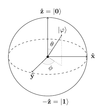
The Y-gate and the Z-gate also change the spin of our qubit electron. But I’d probably need to delve into the esoteric mysteries of the Bloch sphere to really explain how, and I’ve got another gate to go through at the moment…
The Hadamard gate
While the Pauli gates are a lot like classic logic gates in some respects, the Hadamard gate, or H-gate, is a bona fide quantum beast. It shows up everywhere in quantum computing, and for good reason. The Hadamard gate has the characteristically quantum capacity to transform a definite quantum state, such as spin-up, into a murky one, such as a superposition of both spin-up and spin-down at the same time.
Once you send a spin-up or spin-down electron through an H-gate, it will become like a penny standing on its end, with precisely 50/50 odds that it will end up heads (spin-up) or tails (spin-down) when toppled and measured. This H-gate is extremely useful for performing the first computation in any quantum program because it transforms pre-set, or initialized, qubits back into their natural fluid state in order to leverage their full quantum powers.
Other quantum gates
There are a number of other quantum gates you’re bound to run into. Many of them operate on several qubits at a time, leading to 4×4 or even 8×8 matrices with complex-numbered elements. These are pretty hairy if you don’t already have some serious matrix skills under your belt. So I’ll spare you the details.
The main gates that you will want to be familiar are the ones we covered shown in the graph below:

You should know that other gates exist so here’s a quick list of some of the most widely used other quantum gates, just so you can get a feel for the jargon:
- Toffoli gateFredkin gate
- Deutsch gate
- Swap gate (and swap-gate square root)
- NOT-gate square root
- Controlled-NOT gate (C-NOT) and other controlled gates
There are many more. But don’t let the numbers fool you. Just as you can perform any classical computation with a combination of NOT + OR = NOR gates or AND + OR = NAND gates, you can reduce the list of quantum gates to a simple set of universal quantum gates. But we’ll save that deed for another day.
Future gazing through the quantum gateway

As a recent Quanta Magazine article points out, the quantum computers of 2018 aren’t quite ready for prime time. Before they can step into the ring with classical computers with billions of times as many logic gates, they will need to face a few of their own demons. The most deadly is probably the demon of decoherence. Right now, quantum decoherence will destroy your quantum computation in just “a few microseconds.” However, the faster your quantum gates perform their operations, the more likely your quantum algorithm will beat the demon of decoherence to the finish line, and the longer the race will last. Alongside speed, another important factor is the sheer number of operations performed by quantum gates to complete a calculation. This is known as a computation’s depth. So another current quest is to deepen the quantum playing field. By this logic, as the rapidly evolving quantum computer gets faster, its calculations deeper, and the countdown-to-decoherence longer, the classical computer will eventually find itself facing a formidable challenger, if not successor, in the (quite possibly) not too far future.
If you liked this article I would be super excited if you hit the like button 🙂 or share with your curious friends. You can subscribe to this profile and get all my articles sent to you as soon as I write them by clicking the subcribe button! (how awesome?!)
Anyway, thanks again for reading have a great day!